Data Description and EDA
Contents
- Summary
- Downloading and Cleaning Data Set
- EDA: Training Set Image Dimension Stats
- Mean Images
- Preprocessing Code
Summary
We looked at the image dimensions and pixel statistics (per image) and computed the “mean” image across all images.
The (first) mode of each feature was:
 The mode was interesting because although it appeared that there were about 40 mode pixel_means, that was only because several pixel means appeared twice, so the mode value itself was 2, which is very low. It was therefore not particularly informative, but we didn’t expect it to be. In fact, it’s rather remarkable that there were any repeated pixel mean values considering that the mean is the result of averaging thousands of pixels and the images weren’t the same size when this was taken, but still not informative from what we know about image classification.
Other major statistics are shown in the table below, and further down.
train_df.describe()
| breed_id | class | height | width | area | pixel_mean | pixel_median | |
|---|---|---|---|---|---|---|---|
| count | 11999.000000 | 11999.000000 | 11999.000000 | 11999.000000 | 1.199900e+04 | 11999.000000 | 11999.000000 |
| mean | 60.498375 | 3.049754 | 386.289691 | 442.884657 | 1.823229e+05 | 112.143816 | 108.427577 |
| std | 34.642243 | 2.073039 | 127.532994 | 144.615190 | 1.907018e+05 | 27.168085 | 37.636997 |
| min | 1.000000 | 0.000000 | 103.000000 | 97.000000 | 1.150000e+04 | 25.721226 | 3.000000 |
| 25% | 30.500000 | 1.000000 | 333.000000 | 360.000000 | 1.640000e+05 | 94.352833 | 84.000000 |
| 50% | 60.000000 | 3.000000 | 375.000000 | 500.000000 | 1.845000e+05 | 111.822098 | 107.000000 |
| 75% | 90.500000 | 5.000000 | 452.000000 | 500.000000 | 1.875000e+05 | 128.805862 | 130.000000 |
| max | 120.000000 | 7.000000 | 2560.000000 | 2740.000000 | 4.915200e+06 | 230.984512 | 255.000000 |
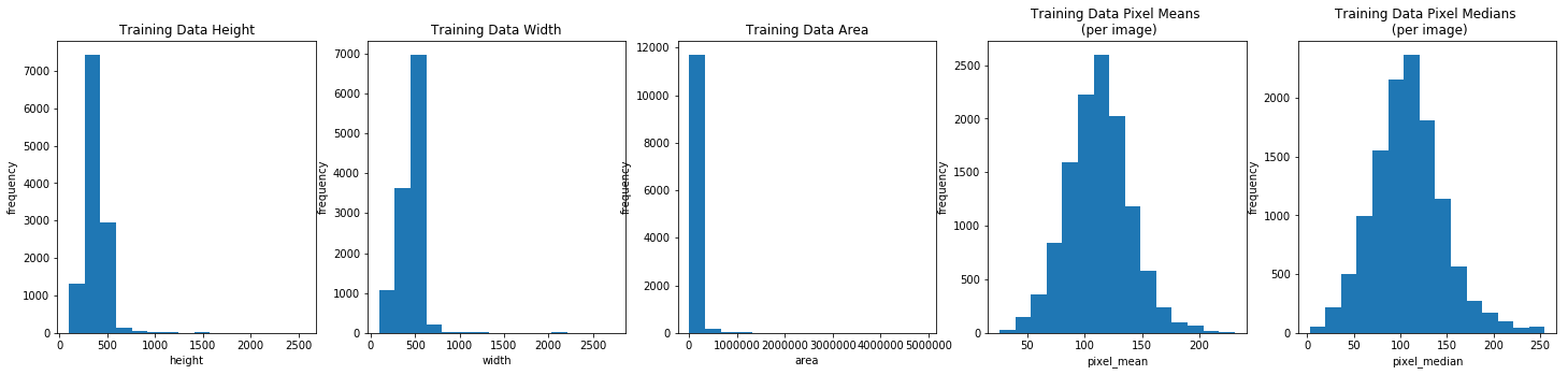
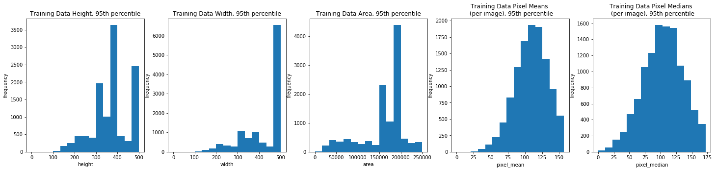
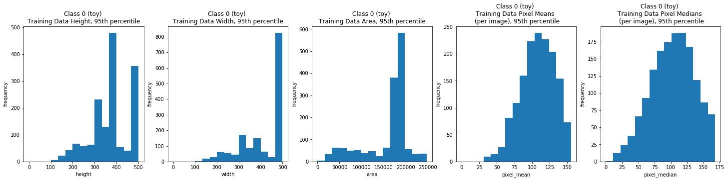
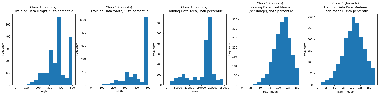
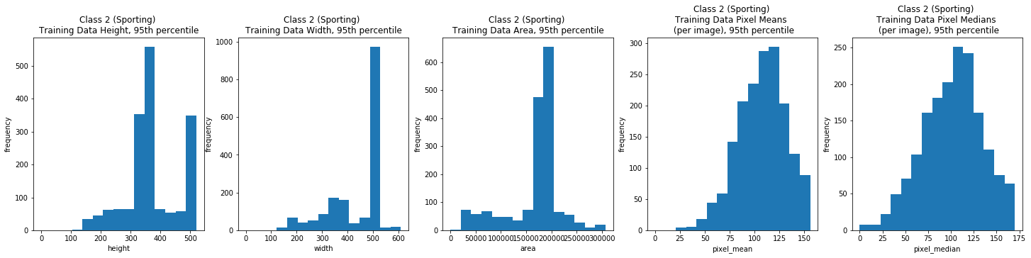
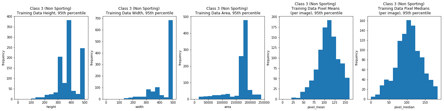
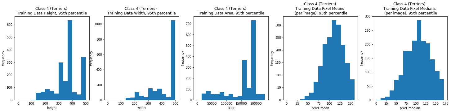
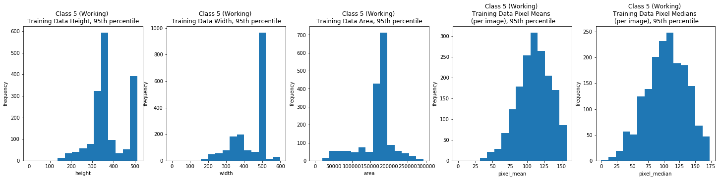
Overall, the image width and height varied greatly, but the majority (the 95th percentile) were typically between 100 and 500 pixels. The per image mean pixel was around 112 and the per image median pixel was around 108 for the entire data set and when we looked at each class individually.
We computed the mean images for the full training set and for each class by composing an image using the mean pixel across all pixel positions in a set of images.
The mean image over all the data is almost the same shade except for a slightly darker center, suggest that the figures are possibly somewhat centered overall. Each class mean images is difference of course but tend to have a central darker spot, some more pronounced than others, which might mean the images in those classes might be easier to group together, or at least to distinguish from the mean images where the central spot is lighter. The “background” color also varies from brown to light green.
The clear outlier is the mean image of the wild dogs set, which suggests that although there are few images like this, they might be more easily distinguished, which would make classifying them more successful.
We found the mean images somewhat interesting but it’s hard to know how informative these trends and differences we notice are.
Downloading and Cleaning Data Set
Data Overview
Our data set is purely jpeg images. There are 12000 training images and 8580 test images. The data set has 120 dog breeds but we will classify by the 7 superbreeds. Of the 120 breeds we have, 5 breeds in the data set that are not classified under a super breed.
“Reconciliation” / Design Choices
There are 5 breeds provided that are not classified under a superclass by the American Kennel Society: the Kelpi, the Appenzeller, the Dingos, the Dholes, and the African Hunting Dog. We decided that although the Kelpie breed and Appenzeller are not officially classified by the AKS, they are frequently classified as herding dogs by other Kennel Societies such as the New Zealand Kennel Society, so for the purposes of this project we decided that they should be classified as herding dogs. This seemed like a reasonable choice given that these dogs are primarily used as herding dogs and therefore if someone is looking for a herding dog, they would be reasonable options, despite not being officially classified as such by the AKS.
The Dingo, Dhole, and African Hunting Dog are all wild dog breeds that are currently endangered. They actually appear rather similar, all medium to large sized dogs that are lean and have short reddish-brown coats and features similar to wolves. We therefore decided to include them as an eighth category, wild dogs. Since the test data will likely include photos of these breeds, we figured it was reasonable to group them together and see what happens, since it would be better that some are classified as wild, if only because the background is never a domesticated setting in the photos of these wild dogs, than their physical similarities.
Cleaning
The images were downloaded and the jpeg file names, labels, and a couple other things were provided in a .mat file. We extracted the relevant information and built a Dataframe with each image file path, breed, breed id, superbreed category (manually compiled by checking the AKS classification for each breed in the data set), and metadata: the image height, width, area, mean pixel, and median pixel.
We had to manually go through each breed and determine which superbreed it belonged to. As mentioned in the “Reconciliation” section, this requried
We had to re-organize the data from the way it was in the dataset, where training and test images are in the same folders, into seperate training and test folders. We therefore have a column with the path for the images before and after they were re-organized.
There was one image, “n02105855-Shetland_sheepdog/n02105855_2933.jpg” that could not be re-sized. Because this was the only one, from both the training and the test set, we chose to remove it from the dataset.
import random
random.seed(112358)

import numpy as np
import pandas as pd
import matplotlib.pyplot as plt

import keras
from keras.models import Sequential
from keras.layers import Dense

%matplotlib inline

import seaborn as sns

from keras import regularizers
import scipy.io
from scipy import stats
from keras.preprocessing.image import ImageDataGenerator, array_to_img, img_to_array, load_img
Using TensorFlow backend.
test_mat = scipy.io.loadmat("test_data.mat")
train_mat = scipy.io.loadmat("train_data.mat")
def unpack_mat(mat, train_or_test):
    df = pd.DataFrame()
    jpgs = []
    scaled_paths = []
    original_paths = []
    breeds = []
    breed_ids = []
    num_datapoints = len(mat[train_or_test][0][0][0])
    for i in range(num_datapoints):
        jpg = mat[train_or_test][0][0][0][i][0][0]
        scaled_path = "images/" + jpg
        original_path = "images_originals/" + jpg
        jpgs.append(jpg)
        scaled_paths.append(scaled_path)
        original_paths.append(original_path)
        temp_arr = mat[train_or_test][0][0][1][i][0][0].strip().split('-')
        breed_str = "-".join(temp_arr[1:]).split('/')[0]
        breeds.append(breed_str)
        breed_ids.append(mat[train_or_test][0][0][2][i][0])
    df['jpg'] = jpgs
    df['breed'] = breeds
    df['breed_id'] = breed_ids
    df['scaled_path'] = scaled_paths
    df['original_path'] = original_paths
    return df
train_df = unpack_mat(train_mat, 'train_info')
test_df = unpack_mat(test_mat, 'test_info')
Superbreed Classification
The dog breeds were manually classified into superbreeds which was then used to add labels to the Dataframes.
toy_ids = np.array([1, 2, 3, 4, 5, 6, 7, 8, 21, 37, 51, 87, 101, 108, 111, 114])
hound_ids = np.array([9, 10, 11, 12, 13, 14, 15, 16, 17, 18, 19, 20, 22, 23, 24, 25,
                      26, 27, 102, 103])
sporting_ids = np.array([28, 55, 56, 57, 58, 59, 60, 61, 62, 63, 64, 65, 66,
                         67, 68, 69, 70, 71])
non_sporting_ids = np.array([45, 50, 54, 73, 95, 98, 109, 110, 115, 116, 117])
terrier_ids = np.array([29, 30, 31, 32, 33, 34, 35, 36, 38, 39, 40, 41, 42,
                        43, 44, 46, 49, 52, 53])
working_ids = np.array([47, 48, 72, 78, 84, 88, 89, 92, 93, 94, 96, 97, 99, 100,
                        104, 105, 106, 107])
herding_ids = np.array([74, 75, 76, 79, 80, 81, 82, 83, 85, 86, 91, 112, 113, 77, 90])
wild_dog_ids = [118, 119, 120]
super_classes = [toy_ids, hound_ids, sporting_ids, non_sporting_ids, terrier_ids,
                 working_ids, herding_ids, wild_dog_ids]
train_df['class'] = np.ones(len(train_df['breed'])) * -1
test_df['class'] = np.ones(len(test_df['breed'])) * -1
for i, super_class in enumerate(super_classes):
    train_df.loc[train_df['breed_id'].isin(super_class), 'class'] = i
    test_df.loc[test_df['breed_id'].isin(super_class), 'class'] = i
train_df.drop(train_df[train_df['class'] == -1].index, inplace=True)
test_df.drop(test_df[test_df['class'] == -1].index, inplace=True)
Adding Features to the Dataframe
X_train = np.array([img_to_array(load_img(path)) for path in train_df['original_path']])
train_df['height'] = [x.shape[0] for x in X_train]
train_df['width'] = [x.shape[1] for x in X_train]
train_df['area'] = train_df['height'] * train_df['width']
train_df['area'] = train_df['height'] * train_df['width']
train_df['pixel_mean'] = [np.mean(x) for x in X_train]
train_df['pixel_median'] = [np.median(x) for x in X_train]
train_df.to_csv("raw_train_df.csv")
test_df.to_csv("raw_test_df.csv")
EDA: Training Set Image Dimension Stats
Full Training Set
train_df = pd.read_csv("raw_train_df.csv", index_col=0)
def pretty_hist(axs, data, xlabel, ylabel, title, truncate_range):
    if truncate_range:
        axs.hist(data, bins=15, range=(0, np.percentile(data, 95)))
    else:
        axs.hist(data, bins=15)
    axs.set_xlabel(xlabel)
    axs.set_ylabel(ylabel)
    axs.set_title(title)
def plot_field_hists(fields, xlabels, ylabels, titles, truncate_range=False):
    num_fields = len(fields)
    fig, axs = plt.subplots(1, num_fields, figsize=(5 * num_fields, 5))
    if truncate_range:
        titles = [x + ", 95th percentile" for x in titles]
    for i, field in enumerate(fields):
        pretty_hist(axs[i], field, xlabels[i], ylabels[i], titles[i], truncate_range)
    plt.show()
def dimension_EDA(df, train_field_xlabels, train_field_ylabels, train_field_titles):
    # 50% is the median
    train_fields = [df[field] for field in train_field_xlabels]
    print('Mode of Each Data Type (can be more than one)')
    display(df[train_field_xlabels].mode())
    display(df.describe())
    plot_field_hists(train_fields, train_field_xlabels, train_field_ylabels, train_field_titles)
    plot_field_hists(train_fields, train_field_xlabels, train_field_ylabels, train_field_titles, truncate_range=True)
train_field_xlabels = ['height', 'width', 'area', 'pixel_mean', 'pixel_median']
train_field_ylabels = ['frequency'] * len(train_field_xlabels)
train_field_titles = ['Training Data Height', 'Training Data Width', 'Training Data Area', 'Training Data Pixel Means \n (per image)', 'Training Data Pixel Medians \n (per image)']
dimension_EDA(train_df, train_field_xlabels, train_field_ylabels, train_field_titles)
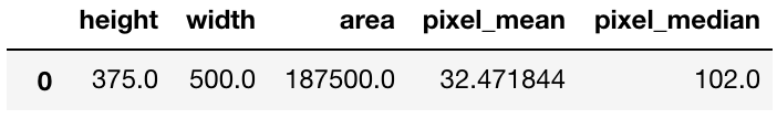
Mode of Each Data Type (can be more than one)
| height | width | area | pixel_mean | pixel_median | |
|---|---|---|---|---|---|
| 0 | 375.0 | 500.0 | 187500.0 | 32.471844 | 102.0 |
| 1 | NaN | NaN | NaN | 74.479744 | NaN |
| 2 | NaN | NaN | NaN | 84.492241 | NaN |
| 3 | NaN | NaN | NaN | 85.132156 | NaN |
| 4 | NaN | NaN | NaN | 87.276344 | NaN |
| 5 | NaN | NaN | NaN | 90.655434 | NaN |
| 6 | NaN | NaN | NaN | 94.959969 | NaN |
| 7 | NaN | NaN | NaN | 99.757095 | NaN |
| 8 | NaN | NaN | NaN | 100.112602 | NaN |
| 9 | NaN | NaN | NaN | 103.104118 | NaN |
| 10 | NaN | NaN | NaN | 103.470612 | NaN |
| 11 | NaN | NaN | NaN | 103.570946 | NaN |
| 12 | NaN | NaN | NaN | 104.854309 | NaN |
| 13 | NaN | NaN | NaN | 108.339966 | NaN |
| 14 | NaN | NaN | NaN | 110.499313 | NaN |
| 15 | NaN | NaN | NaN | 112.021393 | NaN |
| 16 | NaN | NaN | NaN | 113.407219 | NaN |
| 17 | NaN | NaN | NaN | 113.996834 | NaN |
| 18 | NaN | NaN | NaN | 115.102348 | NaN |
| 19 | NaN | NaN | NaN | 115.634087 | NaN |
| 20 | NaN | NaN | NaN | 115.667099 | NaN |
| 21 | NaN | NaN | NaN | 116.413353 | NaN |
| 22 | NaN | NaN | NaN | 118.111633 | NaN |
| 23 | NaN | NaN | NaN | 120.048439 | NaN |
| 24 | NaN | NaN | NaN | 123.686897 | NaN |
| 25 | NaN | NaN | NaN | 128.356125 | NaN |
| 26 | NaN | NaN | NaN | 129.687759 | NaN |
| 27 | NaN | NaN | NaN | 129.876328 | NaN |
| 28 | NaN | NaN | NaN | 131.545944 | NaN |
| 29 | NaN | NaN | NaN | 131.992554 | NaN |
| 30 | NaN | NaN | NaN | 133.000153 | NaN |
| 31 | NaN | NaN | NaN | 139.729370 | NaN |
| 32 | NaN | NaN | NaN | 140.332428 | NaN |
| 33 | NaN | NaN | NaN | 145.873215 | NaN |
| 34 | NaN | NaN | NaN | 148.994186 | NaN |
| 35 | NaN | NaN | NaN | 151.758209 | NaN |
| 36 | NaN | NaN | NaN | 162.024933 | NaN |
| 37 | NaN | NaN | NaN | 162.829636 | NaN |
| 38 | NaN | NaN | NaN | 164.041245 | NaN |
| 39 | NaN | NaN | NaN | 165.401840 | NaN |
| 40 | NaN | NaN | NaN | 167.776276 | NaN |
| 41 | NaN | NaN | NaN | 190.556137 | NaN |
| 42 | NaN | NaN | NaN | 202.729797 | NaN |
| 43 | NaN | NaN | NaN | 208.358734 | NaN |
| breed_id | class | height | width | area | pixel_mean | pixel_median | |
|---|---|---|---|---|---|---|---|
| count | 11999.000000 | 11999.000000 | 11999.000000 | 11999.000000 | 1.199900e+04 | 11999.000000 | 11999.000000 |
| mean | 60.498375 | 3.049754 | 386.289691 | 442.884657 | 1.823229e+05 | 112.143816 | 108.427577 |
| std | 34.642243 | 2.073039 | 127.532994 | 144.615190 | 1.907018e+05 | 27.168085 | 37.636997 |
| min | 1.000000 | 0.000000 | 103.000000 | 97.000000 | 1.150000e+04 | 25.721226 | 3.000000 |
| 25% | 30.500000 | 1.000000 | 333.000000 | 360.000000 | 1.640000e+05 | 94.352833 | 84.000000 |
| 50% | 60.000000 | 3.000000 | 375.000000 | 500.000000 | 1.845000e+05 | 111.822098 | 107.000000 |
| 75% | 90.500000 | 5.000000 | 452.000000 | 500.000000 | 1.875000e+05 | 128.805862 | 130.000000 |
| max | 120.000000 | 7.000000 | 2560.000000 | 2740.000000 | 4.915200e+06 | 230.984512 | 255.000000 |
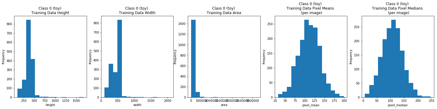
Class 0: Toy Breeds
class_0_train_df = train_df[train_df['class'] == 0]
title_0_prefix = 'Class 0 (toy) \n'
class_0_train_field_titles = [title_0_prefix + t for t in train_field_titles]
dimension_EDA(class_0_train_df, train_field_xlabels, train_field_ylabels,
              class_0_train_field_titles)
Mode of Each Data Type (can be more than one)
| height | width | area | pixel_mean | pixel_median | |
|---|---|---|---|---|---|
| 0 | 375.0 | 500.0 | 187500.0 | 85.132156 | 85.0 |
| 1 | NaN | NaN | NaN | 118.111633 | NaN |
| 2 | NaN | NaN | NaN | 129.687759 | NaN |
| 3 | NaN | NaN | NaN | 164.041245 | NaN |
| breed_id | class | height | width | area | pixel_mean | pixel_median | |
|---|---|---|---|---|---|---|---|
| count | 1600.00000 | 1600.0 | 1600.000000 | 1600.000000 | 1.600000e+03 | 1600.000000 | 1600.000000 |
| mean | 41.62500 | 0.0 | 384.448125 | 429.450000 | 1.741263e+05 | 110.924687 | 106.715312 |
| std | 44.48563 | 0.0 | 122.485669 | 133.053545 | 1.461365e+05 | 26.988897 | 37.484878 |
| min | 1.00000 | 0.0 | 103.000000 | 97.000000 | 1.199000e+04 | 31.965340 | 7.000000 |
| 25% | 4.75000 | 0.0 | 333.000000 | 335.750000 | 1.574850e+05 | 93.075907 | 81.000000 |
| 50% | 14.50000 | 0.0 | 375.000000 | 500.000000 | 1.785000e+05 | 110.878407 | 107.000000 |
| 75% | 90.50000 | 0.0 | 473.500000 | 500.000000 | 1.875000e+05 | 129.197033 | 131.000000 |
| max | 114.00000 | 0.0 | 1662.000000 | 2080.000000 | 3.211520e+06 | 198.951004 | 247.000000 |
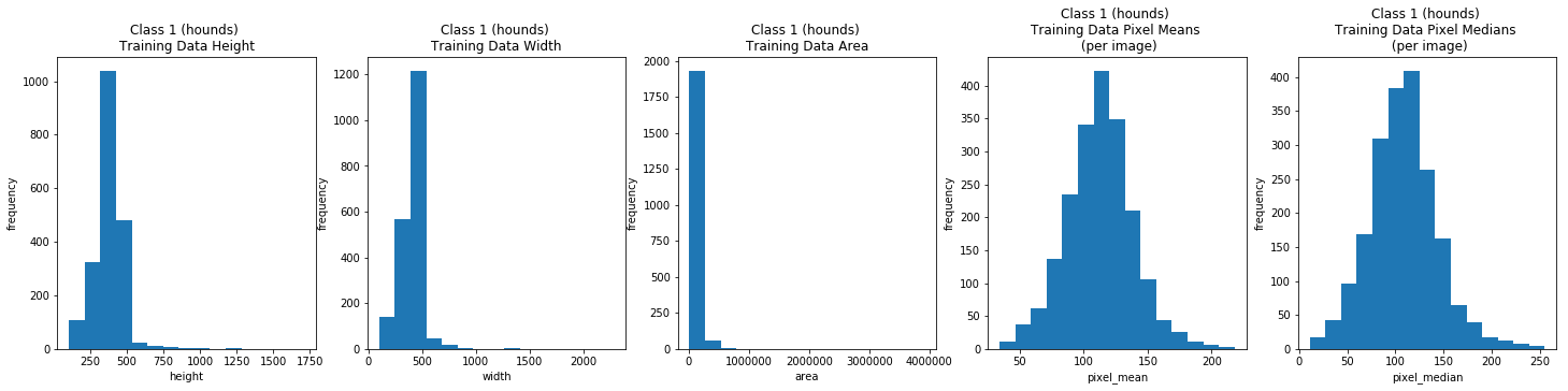
Class 1: Hounds
class_1_train_df = train_df[train_df['class'] == 1]
title_1_prefix = 'Class 1 (hounds) \n'
class_1_train_field_titles = [title_1_prefix + t for t in train_field_titles]
dimension_EDA(class_1_train_df, train_field_xlabels, train_field_ylabels, class_1_train_field_titles)
Mode of Each Data Type (can be more than one)
| height | width | area | pixel_mean | pixel_median | |
|---|---|---|---|---|---|
| 0 | 375.0 | 500.0 | 187500.0 | 87.276344 | 109.0 |
| 1 | NaN | NaN | NaN | 116.413353 | NaN |
| 2 | NaN | NaN | NaN | 123.686897 | NaN |
| 3 | NaN | NaN | NaN | 129.876328 | NaN |
| 4 | NaN | NaN | NaN | 148.994186 | NaN |
| breed_id | class | height | width | area | pixel_mean | pixel_median | |
|---|---|---|---|---|---|---|---|
| count | 2000.00000 | 2000.0 | 2000.000000 | 2000.000000 | 2.000000e+03 | 2000.000000 | 2000.000000 |
| mean | 26.30000 | 1.0 | 377.872000 | 434.038500 | 1.725883e+05 | 112.579294 | 108.389000 |
| std | 25.95278 | 0.0 | 112.941828 | 132.759635 | 1.464921e+05 | 26.134392 | 35.164043 |
| min | 9.00000 | 1.0 | 104.000000 | 100.000000 | 1.150000e+04 | 34.201900 | 11.000000 |
| 25% | 13.75000 | 1.0 | 333.000000 | 350.000000 | 1.403625e+05 | 96.180819 | 86.000000 |
| 50% | 18.50000 | 1.0 | 375.000000 | 500.000000 | 1.780000e+05 | 112.664257 | 108.000000 |
| 75% | 24.25000 | 1.0 | 445.000000 | 500.000000 | 1.875000e+05 | 128.318901 | 128.000000 |
| max | 103.00000 | 1.0 | 1712.000000 | 2288.000000 | 3.917056e+06 | 217.878387 | 255.000000 |
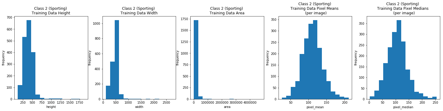
Class 2: Sporting Breeds
class_2_train_df = train_df[train_df['class'] == 2]
title_2_prefix = 'Class 2 (Sporting) \n'
class_2_train_field_titles = [title_2_prefix + t for t in train_field_titles]
dimension_EDA(class_2_train_df, train_field_xlabels, train_field_ylabels,
              class_2_train_field_titles)
Mode of Each Data Type (can be more than one)
| height | width | area | pixel_mean | pixel_median | |
|---|---|---|---|---|---|
| 0 | 375.0 | 500.0 | 187500.0 | 90.655434 | 118.0 |
| 1 | NaN | NaN | NaN | 165.401840 | NaN |
| 2 | NaN | NaN | NaN | 202.729797 | NaN |
| breed_id | class | height | width | area | pixel_mean | pixel_median | |
|---|---|---|---|---|---|---|---|
| count | 1800.000000 | 1800.0 | 1800.000000 | 1800.000000 | 1.800000e+03 | 1800.000000 | 1800.000000 |
| mean | 61.055556 | 2.0 | 393.843889 | 453.330000 | 1.930272e+05 | 110.816578 | 106.490833 |
| std | 9.326826 | 0.0 | 137.025361 | 161.545778 | 2.212782e+05 | 27.520573 | 38.600130 |
| min | 28.000000 | 2.0 | 116.000000 | 108.000000 | 1.296000e+04 | 25.826056 | 3.000000 |
| 25% | 58.000000 | 2.0 | 333.000000 | 375.000000 | 1.665000e+05 | 92.300446 | 81.000000 |
| 50% | 62.500000 | 2.0 | 375.000000 | 500.000000 | 1.875000e+05 | 111.054886 | 106.000000 |
| 75% | 67.000000 | 2.0 | 480.000000 | 500.000000 | 1.875000e+05 | 126.976927 | 128.000000 |
| max | 71.000000 | 2.0 | 1879.000000 | 2740.000000 | 4.745680e+06 | 211.280594 | 255.000000 |
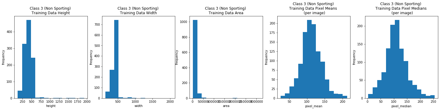
Class 3: Non sporting breeds
class_3_train_df = train_df[train_df['class'] == 3]
title_3_prefix = 'Class 3 (Non Sporting) \n'
class_3_train_field_titles = [title_3_prefix + t for t in train_field_titles]
dimension_EDA(class_3_train_df, train_field_xlabels, train_field_ylabels,
              class_3_train_field_titles)
Mode of Each Data Type (can be more than one)
| height | width | area | pixel_mean | pixel_median | |
|---|---|---|---|---|---|
| 0 | 375.0 | 500.0 | 187500.0 | 74.479744 | 101.0 |
| 1 | NaN | NaN | NaN | 100.112602 | NaN |
| 2 | NaN | NaN | NaN | 133.000153 | NaN |
| 3 | NaN | NaN | NaN | 162.024933 | NaN |
| 4 | NaN | NaN | NaN | 162.829636 | NaN |
| 5 | NaN | NaN | NaN | 190.556137 | NaN |
| breed_id | class | height | width | area | pixel_mean | pixel_median | |
|---|---|---|---|---|---|---|---|
| count | 1100.000000 | 1100.0 | 1100.000000 | 1100.000000 | 1.100000e+03 | 1100.000000 | 1100.000000 |
| mean | 89.272727 | 3.0 | 393.200000 | 449.312727 | 1.834450e+05 | 112.468410 | 109.555909 |
| std | 27.121843 | 0.0 | 115.319479 | 120.120914 | 1.511735e+05 | 29.018573 | 41.689876 |
| min | 45.000000 | 3.0 | 120.000000 | 140.000000 | 2.160000e+04 | 25.721226 | 3.000000 |
| 25% | 54.000000 | 3.0 | 333.000000 | 375.000000 | 1.665000e+05 | 94.456615 | 83.000000 |
| 50% | 98.000000 | 3.0 | 375.000000 | 500.000000 | 1.875000e+05 | 111.383419 | 107.000000 |
| 75% | 115.000000 | 3.0 | 463.500000 | 500.000000 | 1.875000e+05 | 129.573372 | 133.000000 |
| max | 117.000000 | 3.0 | 1926.000000 | 2048.000000 | 3.145728e+06 | 212.646439 | 255.000000 |
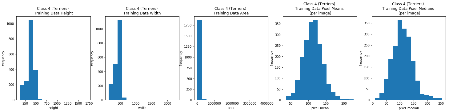
Class 4: Terrier Breeds
class_4_train_df = train_df[train_df['class'] == 4]
title_4_prefix = 'Class 4 (Terriers) \n'
class_4_train_field_titles = [title_4_prefix + t for t in train_field_titles]
dimension_EDA(class_4_train_df, train_field_xlabels, train_field_ylabels,
              class_4_train_field_titles)
Mode of Each Data Type (can be more than one)
| height | width | area | pixel_mean | pixel_median | |
|---|---|---|---|---|---|
| 0 | 375.0 | 500.0 | 187500.0 | 112.021393 | 102.0 |
| 1 | NaN | NaN | NaN | 113.407219 | NaN |
| 2 | NaN | NaN | NaN | 120.048439 | NaN |
| 3 | NaN | NaN | NaN | 128.356125 | NaN |
| 4 | NaN | NaN | NaN | 139.729370 | NaN |
| 5 | NaN | NaN | NaN | 140.332428 | NaN |
| 6 | NaN | NaN | NaN | 151.758209 | NaN |
| 7 | NaN | NaN | NaN | 208.358734 | NaN |
| breed_id | class | height | width | area | pixel_mean | pixel_median | |
|---|---|---|---|---|---|---|---|
| count | 1900.000000 | 1900.0 | 1900.000000 | 1900.000000 | 1.900000e+03 | 1900.000000 | 1900.000000 |
| mean | 39.315789 | 4.0 | 368.577895 | 428.827895 | 1.651163e+05 | 113.146039 | 110.211053 |
| std | 7.065872 | 0.0 | 106.307560 | 121.212291 | 1.179687e+05 | 26.959233 | 37.181410 |
| min | 29.000000 | 4.0 | 120.000000 | 136.000000 | 1.920000e+04 | 37.453369 | 9.000000 |
| 25% | 33.000000 | 4.0 | 332.000000 | 350.000000 | 1.503435e+05 | 94.895241 | 85.000000 |
| 50% | 39.000000 | 4.0 | 375.000000 | 500.000000 | 1.825000e+05 | 112.404808 | 109.000000 |
| 75% | 44.000000 | 4.0 | 400.000000 | 500.000000 | 1.875000e+05 | 129.256058 | 132.000000 |
| max | 53.000000 | 4.0 | 1704.000000 | 2272.000000 | 3.871488e+06 | 227.148422 | 255.000000 |
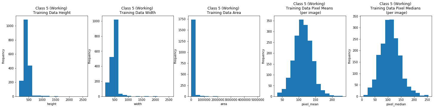
Class 5: Working Breeds
class_5_train_df = train_df[train_df['class'] == 5]
title_5_prefix = 'Class 5 (Working) \n'
class_5_train_field_titles = [title_5_prefix + t for t in train_field_titles]
dimension_EDA(class_5_train_df, train_field_xlabels, train_field_ylabels,
              class_5_train_field_titles)
Mode of Each Data Type (can be more than one)
| height | width | area | pixel_mean | pixel_median | |
|---|---|---|---|---|---|
| 0 | 375.0 | 500.0 | 187500.0 | 108.339966 | 99.0 |
| 1 | NaN | NaN | NaN | NaN | 111.0 |
| breed_id | class | height | width | area | pixel_mean | pixel_median | |
|---|---|---|---|---|---|---|---|
| count | 1800.000000 | 1800.0 | 1800.000000 | 1800.000000 | 1.800000e+03 | 1800.000000 | 1800.000000 |
| mean | 88.833333 | 5.0 | 404.846111 | 457.438333 | 1.998660e+05 | 112.838142 | 108.581667 |
| std | 17.258619 | 0.0 | 152.121098 | 153.338521 | 2.477822e+05 | 27.257844 | 37.257453 |
| min | 47.000000 | 5.0 | 148.000000 | 150.000000 | 2.720000e+04 | 35.495560 | 6.000000 |
| 25% | 84.000000 | 5.0 | 333.000000 | 375.000000 | 1.665000e+05 | 95.017635 | 84.000000 |
| 50% | 93.500000 | 5.0 | 375.000000 | 500.000000 | 1.875000e+05 | 112.156715 | 107.000000 |
| 75% | 100.000000 | 5.0 | 489.000000 | 500.000000 | 1.875000e+05 | 130.954529 | 131.000000 |
| max | 107.000000 | 5.0 | 2560.000000 | 2560.000000 | 4.915200e+06 | 230.984512 | 255.000000 |
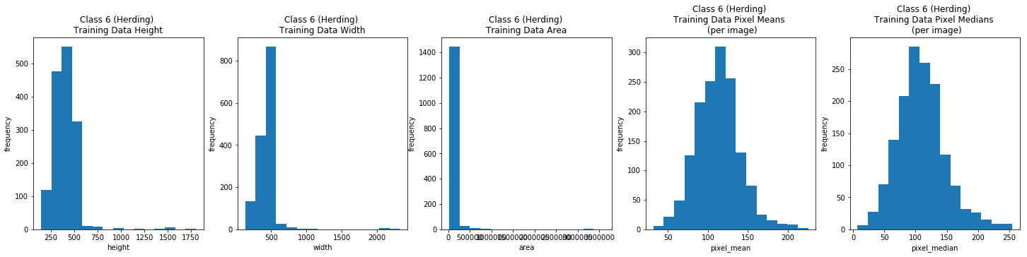
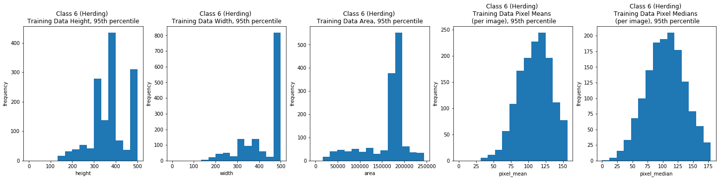
Class 6: Herding Breeds
class_6_train_df = train_df[train_df['class'] == 6]
title_6_prefix = 'Class 6 (Herding) \n'
class_6_train_field_titles = [title_6_prefix + t for t in train_field_titles]
dimension_EDA(class_6_train_df, train_field_xlabels, train_field_ylabels,
              class_6_train_field_titles)
Mode of Each Data Type (can be more than one)
| height | width | area | pixel_mean | pixel_median | |
|---|---|---|---|---|---|
| 0 | 375.0 | 500.0 | 187500.0 | 103.470612 | 95.0 |
| 1 | NaN | NaN | NaN | 113.996834 | 97.0 |
| 2 | NaN | NaN | NaN | 131.545944 | 112.0 |
| 3 | NaN | NaN | NaN | 131.992554 | NaN |
| breed_id | class | height | width | area | pixel_mean | pixel_median | |
|---|---|---|---|---|---|---|---|
| count | 1499.000000 | 1499.0 | 1499.000000 | 1499.000000 | 1.499000e+03 | 1499.000000 | 1499.000000 |
| mean | 85.603736 | 6.0 | 389.637759 | 446.679119 | 1.889250e+05 | 112.617875 | 109.697799 |
| std | 11.627525 | 0.0 | 131.279307 | 168.460965 | 2.409936e+05 | 27.339800 | 38.592978 |
| min | 74.000000 | 6.0 | 143.000000 | 131.000000 | 2.370000e+04 | 31.898178 | 7.000000 |
| 25% | 77.000000 | 6.0 | 333.000000 | 360.500000 | 1.650000e+05 | 93.771652 | 84.000000 |
| 50% | 82.000000 | 6.0 | 375.000000 | 500.000000 | 1.800000e+05 | 112.675102 | 107.000000 |
| 75% | 90.000000 | 6.0 | 452.500000 | 500.000000 | 1.875000e+05 | 128.821785 | 130.000000 |
| max | 113.000000 | 6.0 | 1800.000000 | 2323.000000 | 3.612265e+06 | 225.403122 | 255.000000 |
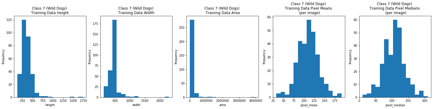
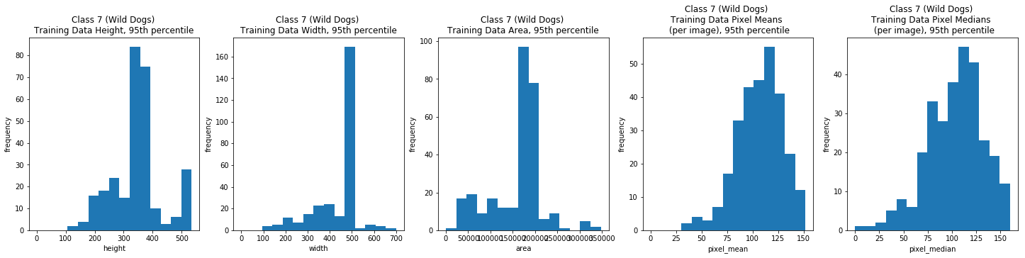
Class 7: Wild Dogs
class_7_train_df = train_df[train_df['class'] == 7]
title_7_prefix = 'Class 7 (Wild Dogs) \n'
class_7_train_field_titles = [title_7_prefix + t for t in train_field_titles]
dimension_EDA(class_7_train_df, train_field_xlabels, train_field_ylabels,
              class_7_train_field_titles)
Mode of Each Data Type (can be more than one)
| height | width | area | pixel_mean | pixel_median | |
|---|---|---|---|---|---|
| 0 | 375.0 | 500.0 | 187500.0 | 32.471844 | 108.0 |
| 1 | NaN | NaN | NaN | 99.757095 | 118.0 |
| 2 | NaN | NaN | NaN | 110.499313 | 120.0 |
| 3 | NaN | NaN | NaN | 115.102348 | 125.0 |
| breed_id | class | height | width | area | pixel_mean | pixel_median | |
|---|---|---|---|---|---|---|---|
| count | 300.000000 | 300.0 | 300.000000 | 300.000000 | 3.000000e+02 | 300.000000 | 300.000000 |
| mean | 119.000000 | 7.0 | 365.673333 | 470.013333 | 1.933222e+05 | 109.633808 | 106.733333 |
| std | 0.817861 | 0.0 | 149.593026 | 184.484221 | 2.617299e+05 | 25.220375 | 32.234854 |
| min | 118.000000 | 7.0 | 132.000000 | 125.000000 | 2.162500e+04 | 32.471844 | 10.000000 |
| 25% | 118.000000 | 7.0 | 301.500000 | 380.750000 | 1.398000e+05 | 93.574894 | 85.000000 |
| 50% | 119.000000 | 7.0 | 334.500000 | 500.000000 | 1.665000e+05 | 110.167782 | 108.000000 |
| 75% | 120.000000 | 7.0 | 375.000000 | 500.000000 | 1.875000e+05 | 123.519602 | 125.000000 |
| max | 120.000000 | 7.0 | 1728.000000 | 2304.000000 | 3.981312e+06 | 190.908478 | 210.000000 |
Mean Images
Pre-processing To Produce Mean Images
X_train_scaled = np.array([img_to_array(load_img(path)) for path in train_df['scaled_path']])
class_dfs = [class_0_train_df, class_1_train_df, class_2_train_df, class_3_train_df, class_4_train_df, class_5_train_df,
             class_6_train_df, class_7_train_df]
class_train_scaled = {}
for i, class_df in enumerate(class_dfs):
    class_train_scaled[i] = np.array([img_to_array(load_img(path)) for path in class_df['scaled_path']])
class_train_cropped = {}
for i in range(len(class_dfs)):
    class_train_cropped[i] = center_crop(class_train_scaled[i])
X_train_cropped = center_crop(X_train_scaled)
X_train_cropped_flattened = np.array([x.flatten() for x in X_train_cropped])
class_train_flattened = {}
for i in range(len(class_dfs)):
    class_train_flattened[i] = np.array([x.flatten() for x in class_train_cropped[i]])
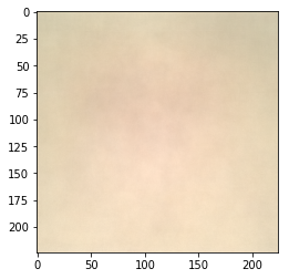
Mean Image for the Full Training Set
aggregate_image = np.mean(X_train_cropped_flattened, axis=0)
array_to_img(aggregate_image.reshape(224, 224, 3)).save("train_aggregate_image", "JPEG")
plt.imshow(array_to_img(aggregate_image.reshape(224, 224, 3)))
<matplotlib.image.AxesImage at 0x1c7cf800b8>
The mean image for the entire data set was almost completely uninformative, although it suggests that the dogs are possibly decently centered and perhaps err on the lighter side, color wise.
Computing the Mean Image per Class
The mean image of each subclass ranged from almost completely uninformative to interesting but not neccessarily helpful in drawing conclusions.
agg_images_by_class = {}
for i in range(len(class_dfs)):
    agg_images_by_class[i] = np.mean(class_train_flattened[i], axis=0)
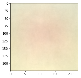
Class 0: Toy Breeds
plt.imshow(array_to_img(agg_images_by_class[0].reshape(224, 224, 3)))
array_to_img(agg_images_by_class[0].reshape(224, 224, 3)).save("train_agg_img_class_0", "JPEG")
This was quite uninformative although the center is just barely pink and the top of the image is slighter darker than the bottom, which might suggest these images are taken closer, so the background is usually seen from the top and the body might be cropped out. This is something we might expect of toy breeds, but this conjecture is not substantiated at all at the moment.
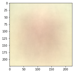
Class 1: Hounds
plt.imshow(array_to_img(agg_images_by_class[1].reshape(224, 224, 3)))
array_to_img(agg_images_by_class[1].reshape(224, 224, 3)).save("train_agg_img_class_1", "JPEG")
This was slightly more interesting than the toy breeds composite image because the color a bit more concentrated, which to us at least suggests that the image similarities are more prominent than that of toy breeds.
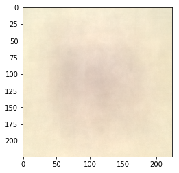
Class 2: Sporting Breeds
plt.imshow(array_to_img(agg_images_by_class[2].reshape(224, 224, 3)))
array_to_img(agg_images_by_class[2].reshape(224, 224, 3)).save("train_agg_img_class_2", "JPEG")
This one’s center is quite concentrated and almost resembles a figure, which is very interesting! It’s slightly more green on the edges, which might suggest more outdoor images, as we would expect from sporting dogs.
Class 3: Non-Sporting Breeds
plt.imshow(array_to_img(agg_images_by_class[3].reshape(224, 224, 3)))
array_to_img(agg_images_by_class[3].reshape(224, 224, 3)).save("train_agg_img_class_3", "JPEG")
This also almost resembles a figure or even a face, which is very interesting! It’s a tad darker than the sporting breeds composite image with no green tone at the edges, which is again is something that might set this class apart.
Class 4: Terrier Breeds
plt.imshow(array_to_img(agg_images_by_class[4].reshape(224, 224, 3)))
array_to_img(agg_images_by_class[4].reshape(224, 224, 3)).save("train_agg_img_class_4", "JPEG")
Quite honestly this could be a very fuzzy terrier if you use some imagination! Just kidding, but the faint reddish-golden brown center is very much like some terriers’ colors. However, since there are many terriers that are white or gray or different colors, this could be misleading, and the models might struggle to use color as good indication when so many colors are represented in many groups, such as the terrier superbreed. The green tones around the borders again suggest perhaps more outdoor photos, whcih we might not expect from terrier breeds since they tend to be domesticated pets.
Class 5: Working Breeds
plt.imshow(array_to_img(agg_images_by_class[5].reshape(224, 224, 3)))
array_to_img(agg_images_by_class[5].reshape(224, 224, 3)).save("train_agg_img_class_5", "JPEG")
This is similar to the non-sporting but slightly more brown and green, which might imply that these images are even more likely to be outdoors and/or the dogs are darker. The center blob also seems just barely less defined, which might suggest greater variety of positions or movements.
Class 6: Herding Breeds
plt.imshow(array_to_img(agg_images_by_class[6].reshape(224, 224, 3)))
array_to_img(agg_images_by_class[6].reshape(224, 224, 3)).save("train_agg_img_class_6", "JPEG")
It’s interesting how concentrated the center spot is. The shape is generally wider than it is tall, which might suggest more pictures from a distance capturing the entire body of the dog, which would make sense for herding dogs since they aren’t as cuddly and perhaps don’t pose as much.
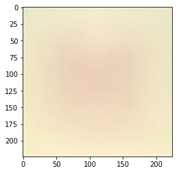
Class 7: Wild Dogs
plt.imshow(array_to_img(agg_images_by_class[7].reshape(224, 224, 3)))
array_to_img(agg_images_by_class[7].reshape(224, 224, 3)).save("train_agg_img_class_7", "JPEG")
We find this the most interesting composite image because it’s the most green with the smallest center brown spot which is on the darker side. To us, because this is the wild dogs class, this is unsurprising because it’s likely that the images are often from a distance and in the wild, which could explain the smaller “body” and abundance of green and dark brown tones. Despite being wild dogs, it might be that their general background is quite similar, since the homes of domestic dogs might have much more variety than a natural backdrop.
Preprocessing Code
Preprocessing consists of resizing all images to 224 x 224 and scaling all pixels (dividing by 255). To resize, we first resize the smaller side to 224, and then take a random crop of 224 pixels (for the training set) or the center crop of 224 pixels (for the test set).
Resize First Side
To resize the first side of all the images in the training data, run ‘python resize_smaller_side.py’
Resize Second Side
def random_crop(list_of_np_arrays):
    cropped = []
    for np_array in list_of_np_arrays:
        w, h = np_array.shape[1], np_array.shape[0]
        img = array_to_img(np_array, scale=False)
        top = random.randint(0,h-224)
        bottom = top + 224
        left = random.randint(0,w-224)
        right = left + 224
        img = img.crop((left, top, right, bottom))
        cropped.append(img_to_array(img))
    return np.array(cropped)

def center_crop(list_of_np_arrays):
    cropped = []
    for np_array in list_of_np_arrays:
        w, h = np_array.shape[1], np_array.shape[0]
        img = array_to_img(np_array, scale=False)
        img = img.crop((w/2  - 112, h/2 - 112, w/2 + 112, h/2 + 112))
        cropped.append(img_to_array(img))
    return np.array(cropped)

#Usage:
Scaling
def scale_pixels(list_of_np_arrays):
    scaled_arrays = []
    for np_array in list_of_np_arrays:
        scaled_arrays.append(np_array / 255)
    return np.array(scaled_arrays)
#Usage: